Three-point Test Cross
A three-point test cross involves crossing an individual who is heterozygous for three genes with a fully recessive tester:
AaBbCc x aabbcc
Or
a+ab+bc+c x aabbcc
The idea of a test cross is that when you observe the phenotype of a specific progeny you know what alleles that progeny inherited from the heterozygote. This is possible because you know that the a, b and c alleles were inherited from the tester. This means that if a progeny has all three dominant phenotypes (we will write this as [ABC]) then you know that it inherited A, B and C alleles from the heterozygote. If a progeny has the [ABc] phenotypes then you know it inherited A, B and c alleles from the heterozygote. This relationship between progeny phenotype and the gametes inherited from the heterozygote parent is exploited in the calculations below.
Three-point test crosses and Linkage
Three-point test crosses are often used in studies of linked genes. They are a convenient way to measure Recombination Frequency for the genes involved and then generate a linkage map from the data.
Here is how it is done:
Say that there are three genes in corn designated by the letters P, V and B. There is a wild type allele for each (p+, v+ and b+) as well as a recessive mutant.
The phenotype associated with each is:
| Gene | Dominant | recessive |
| P(urple) gene | Purple leaves | green leaves |
| V(iral) gene | Sensitive | resistant |
| B(rown) gene | Brown seed | plain seed |
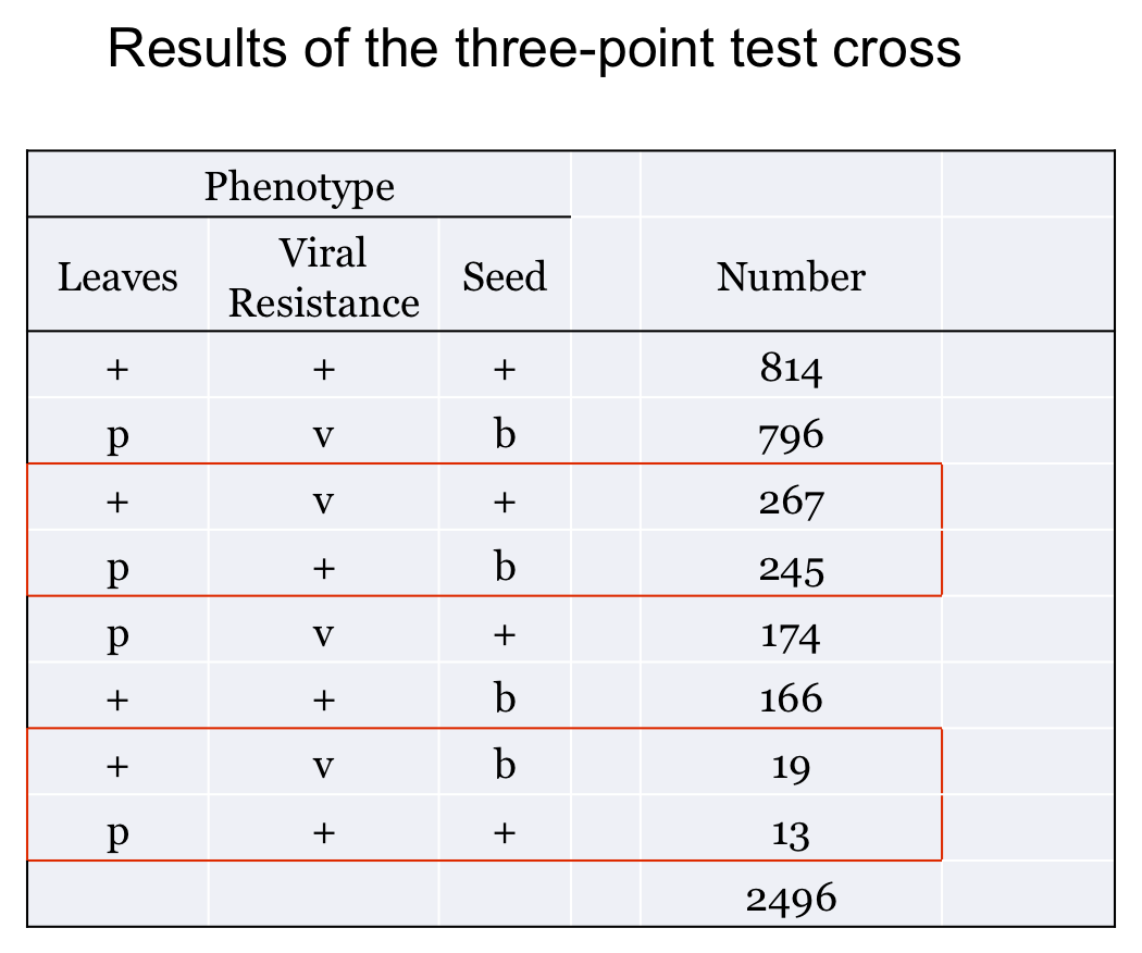
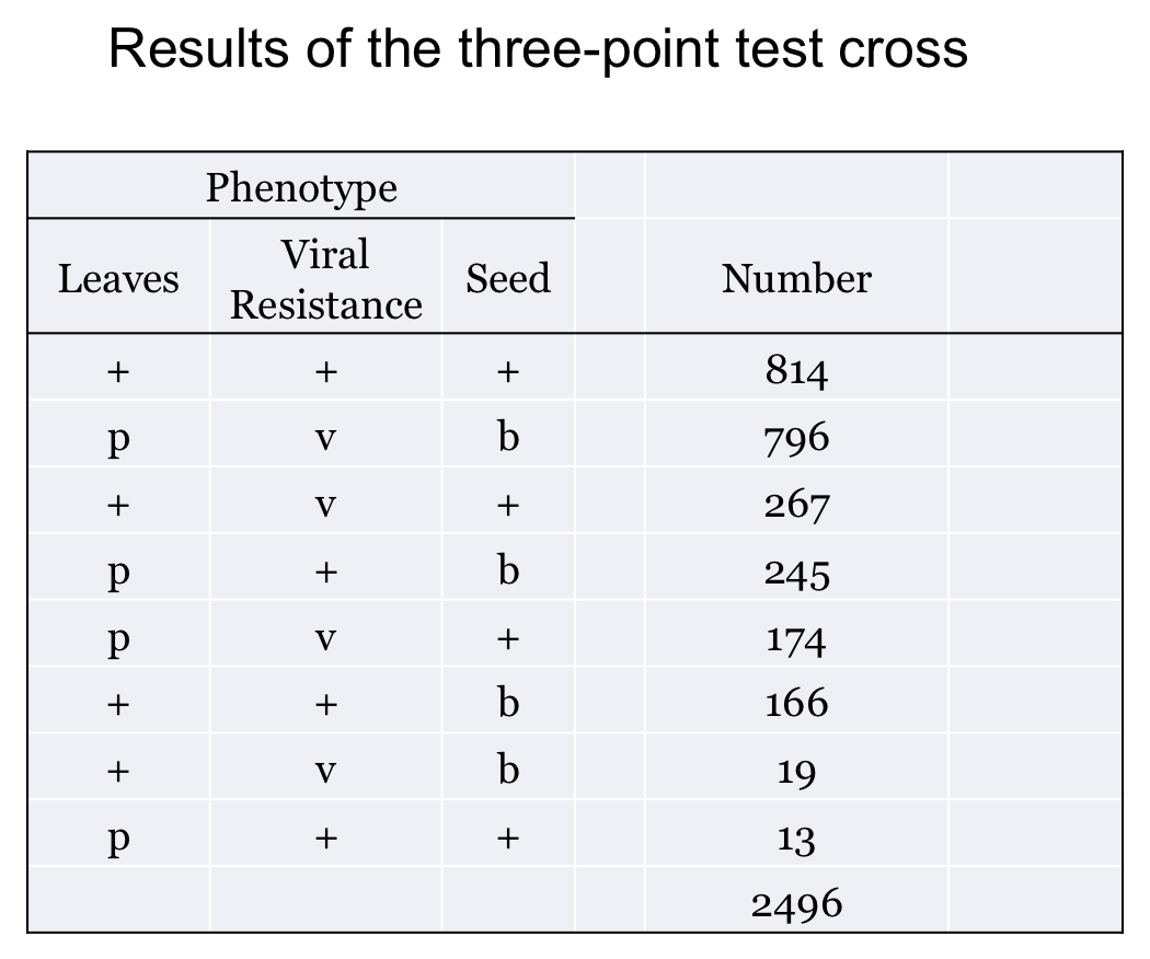
You perform a three-point test cross, p+pv+vb+b x ppvvbb and get the results shown here:
|
|
Before we start on the solution you should take note of a few things. First, the progeny form pairs of phenotypes that are "complements" of one another. This means that where a dominant phenotype shows up in one the recessive shows up in the other. Two such pairs are indicated here:
|
|
Within each pair of complements the numbers are roughly equal. This is because of the fact that these pairs result from the segregation of chromosomes in the heterozygote.
Second, we do not use the terms cis or trans for the entire arrangement of alleles. These terms only apply to gene pairs. So, in the genotype p+vb+/pv+b the P and V genes are in trans but the P and B genes are in cis.
Third, just because we have written the genes in a particular order does NOT necessarily mean that they occur in that order along the chromosome. Obviously we have to write them down in some order - just don't let it mislead you. We will not know the actual order until after the analysis.
Now to the solution. There are a couple of approaches to analyzing three-point test cross data, but the following procedure is probably the easiest:
1. Determine the allele combinations in the heterozygote. These are the parental allele combinations (in the heterozygote). For example p+v+b+/pvb or p+vb+/pv+b. Any arrangement is possible as long as each gene is heterozygous.
How do you know the parental combination? Well, either it tells you in the question or you can determine it from the cross used to generate the heterozygote. The other trick is that one pair of progeny phenotypes will be observed in much greater numbers than any other. This pair tells you the two parental arrangements. (of course, they should be complementary!)
In our example, the p+v+b+ and pvb progeny are by far the most common so these tell us the parental allele combinations.
2. Find the total number of progeny. Pretty straightforward. In our example it is 2496.
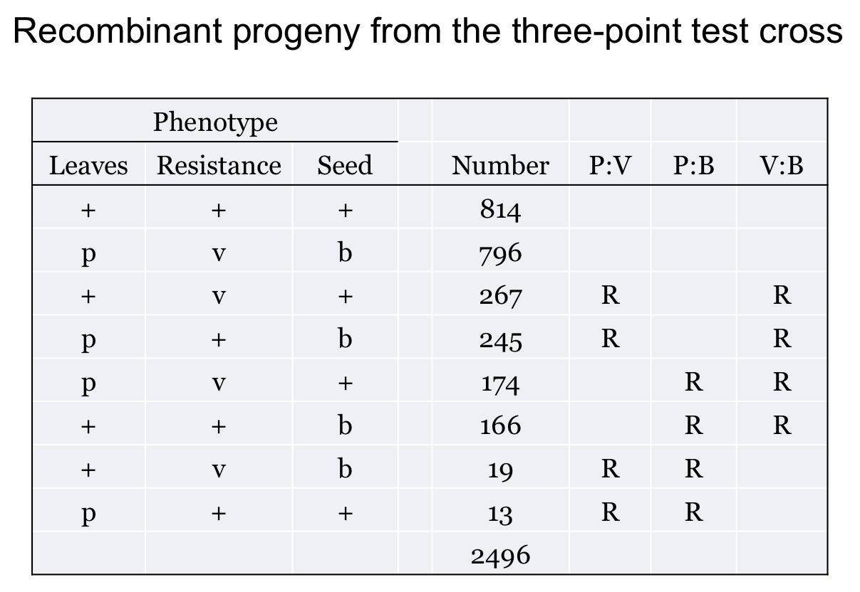
3. Classify each progeny as Parental or Recombinant for each gene pair. Above in (1) we determined the parental combination. Now, for each gene pair determine the parental arrangement. Given what we found in (1), each gene pair is in cis. Therefore, every progeny phenotype can be categorized as being Parental or Recombinant for each gene pair.
This is shown here. R indicates a Recombinant combination, if it is blank then it is Parental.
|
|
4. For each gene pair calculate Recombination Frequency. For that gene pair, count the number classified by R (in step 3) and divide by the total from step 2.
For example, for the P to V genes you should get 544/2496 = 21.8% RF (= 21.8 cM).
You should also find that the V to B distance is 34.1 cM and the P to B distance is 14.9 cM.
5. Draw your map. This should be easy to do. The two genes with the highest RF are the furthest apart, the other is in the middle. In our example, V and B are the furthest apart. Here I have rounded off the RF values.
So, our map is: |-- V -- 22 cM -- P -- 15 cM -- B --| which is NOT the order we originally wrote!
6. Deal with double crossovers. You should see that your numbers don't quite add up; 21.8 cM + 14.9 vcM is not equal to 34.1 cM!
This discrepancy is due to double crossovers and it is easy to deal with once you have your map. Double crossovers are those cases when, during meiosis, there is a cross over between (in our example) the V and P genes and ALSO between the P and B genes. The result is recombination between each of these pairs but the two crossovers cancel each other out when dealing with the V and B genes.
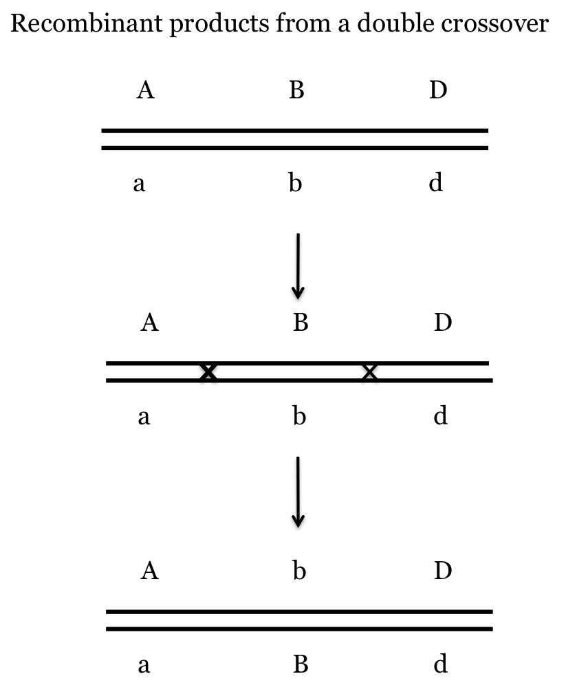
The idea of canceling out can be seen in the next figure. Notice how the products of the double crossover are [A, D] which is parental, but [A, b] and [b, D] which are recombinant. Therefore, using our approach the progeny from these gametes will count as Recombinant for A and B and Recombinant for B and D but as Parental for A and D. This results in an underestimate of the genetic distance between the outside genes.
|
|
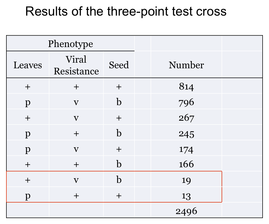
In our example, the progeny resulting from double cross overs are indicated in the Table.
|
|
This is actually not a problem for us. All it means is that the distance we calculate for the two outside genes is a slight underestimate of the distance we get from adding up the two internal distances. However, this does not generate a problem for determining the gene order, and thus the map, from the RF values we do calculate. Also, the actual Map Distance between the external genes, which in our example is 36.7 cM, is easy to calculate once the map is complete simply by addition together the two internal distances.
Although the double crossovers do not generate a problem for us we can "correct" for them once we have the map. We do this by calculating the total number of crossovers between the two outside genes. We had originally counted the double crossovers as parental for V and B, but we can now account for them with the following calculation:
Rec. Freq. (Outside Genes) = [# Recombinants (single x-over) + 2 * # Recombinants (double x-over)] / # Progeny
= [267 + 245 + + 174 + 166 + 2 * (19 + 13)] / 2496
= 916 / 2496
= 36.7 cM
What is important is that, although our method will underestimate the outside gene distance, it still allows us to generate an accurate map. What you should see is that the correction is mathematically guaranteed to give us the same value as adding the two internal distances. Therefore, leaving it until the end, or not even doing it, is just fine. However, it does provide a good lesson for the understanding of how RF can be affected by multiple crossovers between genes which can become important in other sections.